© 2004 Robert A. Freitas Jr. and Ralph C. Merkle. All Rights Reserved.

Robert A. Freitas Jr., Ralph C. Merkle, Kinematic Self-Replicating Machines, Landes Bioscience, Georgetown, TX, 2004.

5.9.2 Strategies for Exponential Kinematic Self-Replication

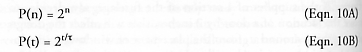
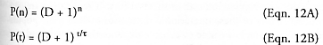
Fibonacci’s rabbits must wait one time period to mature before they can begin replicating, markedly slowing the population growth rate. But consider a replicator that is a fully functional adult device from birth and can immediately begin the construction of its own daughter without waiting. Such entities may be called “birth-mature replicators.” At the end of the first cycle (n = 1), there are 2 adult devices, the first having constructed the second. At the end of the second cycle (n = 2), there are 4 adult devices, each of the first-cycle devices having constructed their own copies. The series progression, starting from the end of the first replication cycle, is therefore 2, 4, 8, 16, ..., and so the population of birth-mature replicators follows the simple exponential law:

after n cycles have elapsed; P(n) > F_end(n) for all n > 0. Note that the replicator population can be restated as P(t) in terms of t, the total elapsed time since replication began, and the replication time t, the time a replicator requires to complete a replication cycle.

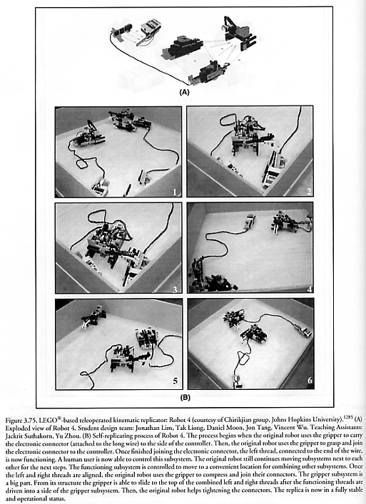
Even faster population growth P_fast(n) > P(n) may be obtained by placing each completed subunit of the daughter that is currently being built into full productive use immediately, instead of waiting for the final completion of the daughter device. There are many design configurations where something close to this can be achieved efficiently, most notably the factory models (e.g., Sections 3.11, 3.13.2.2, 3.15, 4.9.3, 4.14, and 5.9.6) wherein more specialized subunits within the factory (e.g., an individual lathe) could be pressed into immediate service prior to completion of the entire factory (Freitas and Gilbreath [2], Section 5.3.5 at p. 218; see also “Operating-Subsystem-in-Process Replication”, Section 5.1.8), and there has been at least one experimental demonstration of this by the Chirikjian group (see “Robot 4” in Section 3.23.2 and Figure 3.75).

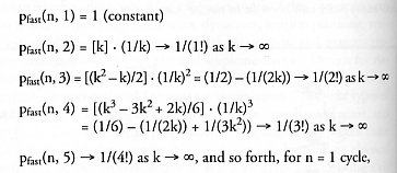
Let us consider that the replication cycle is divided into k time segments, such that at the end of each time segment all components built during that time segment can begin fully contributing to replicative activities. For k = 1, the base population of fast replicators p_fast(1) = 1 + 1 (replicator plus daughter) = 2 devices, at the end of the n = 1 cycle. For k = 2, at the end of half a cycle, the original replicator has built half a daughter, and that half now enters service. By the end of the replication cycle, the second half of the daughter has been built by the original replicator and the daughter has also had half a cycle to begin construction of a granddaughter device, which is now one-quarter completed; hence p_fast(1) = 1 + 2·(1/k) + 1·(1/k)² = 2.25 devices. For k = 3, p_fast(1) = 1 + 3·(1/k) + 3·(1/k)² + 1·(1/k)³ = 2.37 devices; for k = 4, p_fast(1) = 1 + 4·(1/k) + 6·(1/k)² + 4·(1/k)³ + 1·(1/k)⁴ = 2.44 devices produced during the n = 1 replication cycle. Since the coefficients of each term are horizontal elements of Pascal’s triangle,* which is a two-dimensional number array constructed by sequential addition much like Fibonacci numbers, it can be shown that p_fast(n) = p_fast(n, 1) + p_fast(n, 2) + ... is an infinite series with the individual terms:

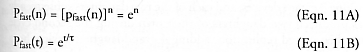
whose sum converges to p_fast(n) = 1 + 1/(1!) + 1/(2!) + 1/(3!) + 1/(4!) + ... = e = 2.71828...., for n = 1 cycle. Hence:

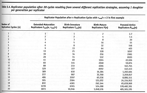
in the limit as k → ∞, providing another example of exponential growth. Table 5.4 shows the replicator populations resulting from each of the four modes of replication discussed so far: P_fast(n) > P(n) > F_end(n) > F_mat(n, t_mat/t) for n > 3, and after n = 20 replication cycles, [P_fast(20) ~ 10⁹] >> [P(20) ~ 10⁶] >> [F_end(20) ~ 10⁴] > [F_mat(20, t_mat/t = 2) ~ 10³]. Clearly, the choice of replication strategy produces significantly different population growth rates.

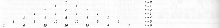
* The French mathematician Blaise Pascal described a triangular arrangement of numbers – now called Pascal’s Triangle [2843] – that are useful in algebra and probability theory, in which every number in the interior of the triangle is the sum of the two numbers on either side directly above it:

So far we have considered only replicators that produce a single offspring during each replication cycle. If each replicator can produce D daughters per generation – i.e., a “litter” of D offspring per pregnancy, rather than just a single daughter per pregnancy – then for birth-mature replicators:*

* Star Trek’s fictional “Tribbles” are furry earless rabbits that are said to be “born pregnant” and to produce a litter of D = 10 offspring every 12 hours [2844], so three days of unconstrained replication (n = 6) produces a total population of 1,771,561 animals, using Eqn. 12 for birth-mature replicators.

and for prenatal-active replicators:

after n cycles have elapsed, for D > 0, n > 0. While D > 1 gives much higher populations at any given number of cycles than for D = 1, the replication time t will correspondingly be longer for D > 1 because more mass must be replicated in each cycle. In the simplest case, making twice as many daughters requires replicating twice as much mass, which takes twice as much time at a constant production rate, hence t / t₀ ~ D, where t₀ is the replication time for D = 1 daughter per litter. In this simple case, Eqns. 12 and 13 predict that the population-maximizing strategy is to minimize the number of daughters, i.e., D = 1 yields the fastest population growth rate. What if the manufacturing time per daughter can be made smaller for additional daughters by some technical means (e.g., “cheaper by the dozen”; see Section 5.9.6)? The population growth-neutral replication time dependency is t_neutral / t₀ = log₂(D + 1) for birth-mature replicators and t_neutral / t₀ = 1 + log_e(D) for prenatal-active replicators. That is, if t = t_neutral, then choosing any number of daughters per litter gives the same population growth rate. If t > t_neutral, as where t / t₀ ~ D in the simplest case above, then minimizing the number of daughters per litter maximizes the population growth rate. If t < t_neutral, then maximizing the number of daughters per litter maximizes the population growth rate. Tradeoffs among these variables should be more systematically investigated.

In the case of the Merkle Cased Hydrocarbon Assembler (Section 4.10.2) where the parental birth-mature replicator is destroyed after each generation is completed, from Eqn. 12A the replicator population is only P(n) = Dⁿ after n generations with D daughters per generation. If a constant time is assumed to be required to assemble each daughter machine and if there is no lag time between completing one cycle and beginning the next one, then the total number of replication cycles N = nD, hence P(n) = D^N/D. Taking the derivative with respect to D using the general power rule for differentiation, (∂/∂D)P(n) = (1 – ln(D)) · D^((1/D)-2) which goes to zero when the replicator population P(n) is maximized. For D > 0, then (∂/∂D)P(n) = 0 occurs when 1 – ln(D) = 0; that is, when D = e = 2.718... ~ 3, the optimum number of daughters. (Thanks to C. Phoenix for inspiring this analysis.)

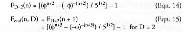
In the case of birth-immature replicators (e.g., Fibonacci rabbits or human beings), Darbro and von Tiesenhausen [1090] report that if these replicators are allowed to produce D = 2 pairs of offspring per replication cycle instead of just D = 1 pair of offspring, and keeping t_mat/t = 1, then the original “rabbit formula” (Eqn. 4) for total rabbit-pair population F_end(n, D) after n replicative cycles becomes:

For birth-immature replicators with D > 2, “some similar expressions may be derived [but] they are not so compact” [1090]; some formulations have previously been addressed by Hoggatt and Lind [2845]. The authors are unaware of any similar calculations for extended-maturation replicators (t_mat/t > 1) with D > 1 that have been published.

Interestingly, a similar set of formulas applies in the financial world, wherein the growth of a given quantity of money is dependent upon the interest rate, “discount” rate, or rate of return. For example, if an initial quantity of money $₀ earns an annual interest rate of i and is allowed to compound m_$ ≥ 1 times every year, then the quantity of money after a period of Y years is given by $(n) = $₀ · (1 + i/m_$)ⁿ where n = m_$Y is the number of compounding periods elapsed. In the case of a 100% annual interest rate, the original money doubles or “replicates” itself in one year if compounded only once (m_$ = 1), so i = 1.00 and $(n) = $₀ · (1 + (1/m_$))ⁿ = $₀ · 2ⁿ which is equivalent to Eqn. 10 for birth-mature replicators.* In the limit as compounding becomes continuous (m_$ → ∞), then $(n) = $₀ · eⁿ which is equivalent to Eqn. 11 for prenatal-active replicators. In a properly functioning capitalist economy, money acts much like a self-replicating entity, with an initial invested amount producing more of itself over time.

* According to one version [2988-2990] of an ancient parable on compound interest, after a wise man performs a useful service for a king in India and the king insists that the man name a reward, the wise man agrees to take one grain of rice for the first square on the king’s chessboard on the first day, two grains for the second square on the second day, and so on, doubling the amount daily for all 64 squares of the chessboard. The king, too proud to admit his inability to calculate the sum total of the gift, foolishly grants the wish, at least until it becomes clear that it will wipe out the royal granary (he has committed to deliver 2⁶⁴ = 18,446,744,073,709,551,616 grains of rice or ~1 trillion metric tons, or 2600 times the world production of milled rice in 2002 [2991]). Finally, despite his pride the king takes back his repayment, justly embarrassed because of his stupidity and the wise man’s obvious generosity in not wanting repayment in the first place. Other versions of this folktale have similar events occurring in China [2992], Persia, or Japan, and there are darker accounts in which the king is outsmarted by a peasant who is ordered killed when the king discovers his own error.

Last updated on 1 August 2005