© 2004 Robert A. Freitas Jr. and Ralph C. Merkle. All Rights Reserved.

Robert A. Freitas Jr., Ralph C. Merkle, Kinematic Self-Replicating Machines, Landes Bioscience, Georgetown, TX, 2004.

5.9.3 Limits to Exponential Kinematic Self-Replication

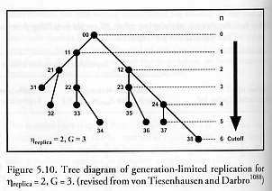
All of the foregoing scenarios assume that a fecund replicator continues replicating indefinitely – that is, that the replicators are immortal. From a pragmatic engineering perspective it is likely that a fecund replicator will become senescent or damaged after some finite number of replications, or, even if still healthy, might be diverted to nonreplicative activities once the population of replicators has grown large enough. In 1980, both von Tiesenhausen and Darbro [1088, 1090] and Valdes and Freitas [1089] examined artificial self-replicating systems in which each replicator device is assumed to produce only a fixed number h_replica of replicas (constructed at the rate of one daughter per replicative cycle per parent replicator, i.e., litter size D = 1) for a fixed number of generations G, after which time replicative activity ceases and useful production (i.e., nonreplicative activity) begins. In this case, the total population P(h_replica, G) of replicators at cutoff, when replication stops, is given by:

where the number of replication cycles required to reach cutoff is n = G h_replica. and the time to reach cutoff is t_cutoff = nt, where t is the replication time, the units of time required for each replication cycle to be completed [1088-1090]. Figure 5.10 shows a tree diagram of one case of generation-limited replication [1088], and McCord [1092] has created a matrix notation to efficiently represent the state vector of the generation-limited replicas.

We can also examine the limited-replica instance of Eqn. 12, wherein h_replica = D. That is, each replica gets only one pregnancy, produces a single brood of D daughters, and then stops any further replicative activities; each daughter also gets one pregnancy, and so forth. Von Tiesenhausen and Darbro [1088, 1090] find that the total population P_onebrood(n) after n replicative cycles is given in this case by:

For example, taking h_replica = 2 then after n = 2 replicative cycles, P_onebrood(2) = 7 because the original replicator has produced two daughters during the first cycle and then ceased further replication, making 3 extant devices, and each of the two daughters subsequently has produced two daughters of their own during the second cycle and then ceased replication, adding 4 granddaughter devices for a total of 7 devices extant. This may be contrasted with the case of unlimited broodnumber assumed for Eqn. 12, which for D = 2 and n = 2 gives P(2) = 9 because the original replicator can produce another two daughters during the second cycle, adding 2 more devices to the previous total of 7.

Continuous exponential growth is only possible for populations of replicators having (1) access to an abundance of material, energy, and information inputs, (2) unrestricted disposal of material and energy outputs so that these outputs will not interfere with replicative activities, (3) no geometric constraints on the positioning or mobility of the physical replicator or any of its external support facilities, and (4) freedom from excessive inherent mortality (i.e., mean replicator lifespan < t_mat or t), predation, or other programmatic or external restrictions on replication rate or survivability. If replicators are constrained in any of these operational dimensions, then their population may no longer be able to achieve exponential growth and may instead revert to polynomial* or other patterns of growth, or may even cease to grow at all.

* A power law relates one variable to another raised to a constant power, with the general form of y = x^a, where y and x are variables and a is a constant exponent or “power.” A polynomial in x is a sum of various powers of x and their positive or negative multiples. The highest power of x which occurs in an equation of growth is called the degree of the polynomial. A polynomial of degree 1 (y = ax + b) is called linear; a polynomial of degree 2 (y = ax² + bx + c) is called quadratic; a polynomial of degree 3 (y = ax³ + bx² + cx + d) is called cubic, and so forth. If the polynomial has an infinite number of powers of x whose terms are summed together, it becomes an “exponential” or “power” series. We have seen an example of a power series in Eqn. 11 in which the sum of the series reduces to the general form of y = a^x, where y and x are variables and a is a constant base, in this case the natural logarithm e.

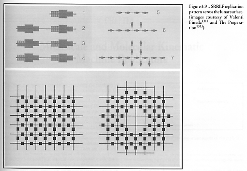
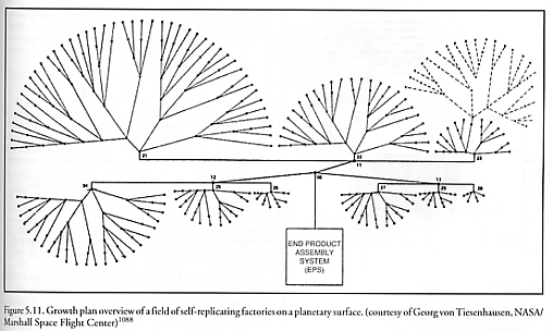
For example, exponential growth is not possible for indefinite periods of time on a surface which is the sole fixed source of vital material inputs to a population of replicators (e.g., a lunar factory metabolizing only in situ lunar materials), if population growth occurs via symmetrical radial expansion without shape change or re-siting of units [1073]. Plane surfaces have only a small number of allowed symmetric repetitive structures [2846]. On such surfaces the only possible shapes allowed for contiguous identical units are shapes whose symmetry angles in revolution are 120^o, 90^o, and 60^o – angles given by 360^o/p for p = 3, 4, or 6 corresponding to triangular, square, or hexagonal symmetry [1073]: “For these shapes the exponential growth rate (2)ⁿ stops at n = 3, 4, and 5 respectively, where n denotes the number of generations. Once p sides are used up in casting off replicas, no doubling can occur by the unit whose sides are closed off. For a hexagonal SRS (replicator), the sixth side is closed off by neighbor growth before the SRS can produce a sixth replica. Exponential growth on the surface of a planetary body is thus possible only for a few generations. After sufficient generations, replication on a surface can continue only by those replicating systems at the boundary of the SRS population (Figure 3.91). The size of the boundary increases as the square root of the population area and the number of systems, thus the growth is given by a quadratic rule” of the form P = An² + Bn + C, where P is the total number of self-replicating systems (SRS), n is the number of replicative cycles elapsed, and A, B, and C are constants defined by geometric and replicator design constraints. (Taneja and Walsh [1073] give one example of a 4-fold (adjacent squares) symmetrical layout strategy with A = 2, B = -6, C = 8.) The transition from exponential to polynomial population growth can be postponed by placing initial growth nuclei at numerous well-separated locations (Figure 5.11) so that replicators will not interfere with resource scavenging and other replicative activities of neighboring devices. But as the interior area is filled in, exponential growth is no longer possible as the maximum carrying capacity of the resource environment is approached – replication has become resource-limited.

In population dynamics, this situation is often modeled using a logistic equation of the form:

where N(t) is the number of replicators at time t, R_max is the maximum unconstrained population growth rate (net of reproduction and mortality), and K is the maximum replicator carrying capacity of the environment. If N(t) < K and approaches K, growth slows to zero as population rises to a plateau, producing the familiar S-shaped logistic curve.

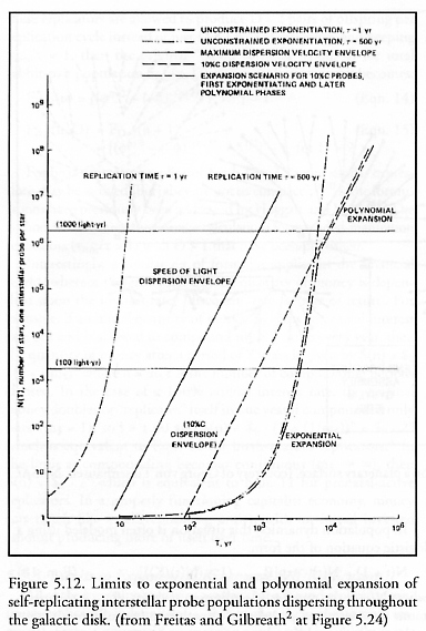
Freitas (Advanced Automation for Space Missions [2], Section 5.4.4) has also pointed out that no expanding population can disperse faster than its medium will permit, regardless of the speed of manufacture. In the context of a hypothetical far future space exploration program, an expanding spherical population of self-replicating interstellar probes can exhibit exponential population growth of N(t) = e^t/t if new replicators are produced relatively slowly so that envelope expansion velocity does not constrain dispersal (in which case other constraints will come into play). However, if unit replication is so swift that multiplication is unconstrained by replication time, then the population can grow only as fast as it can physically disperse – that is, only as fast as the expansion velocity of the surface of the spherical outer envelope – or according to:

where V is peak dispersion velocity for individual replicators at the periphery and d is the number density of useful sites for replication (e.g., uninhabited solar systems). Figure 5.12 shows the transition from exponential to polynomial (a cubic polynomial, in t) population growth when slow (t = 500 yr) but exponentiating replicators encounter a V = 10% c (c = speed of light) velocity constraint during their expansion; replication in this case is mobility-limited.

Replication can also be mortality-limited, whether intrinsic to the system or externally imposed. For instance, the exponential model of self-replication in population dynamics, commonly associated with Thomas Robert Malthus (1766-1834) [2847], assumes that replication is continuous (no seasonality), all replicators are identical (no age structure), and environmental resources are unlimited, in which case the replicator population as a function of time is:

where R = (b – m) is called the Malthusian parameter, the instantaneous rate of natural increase, or the population growth rate. R can be interpreted as the difference between the birth rate (replication) and the death rate (mortality), with birth rate b defined as the number of offspring produced per unit time, per member of the population, and death rate m defined as the number of replicator deaths per unit time, per member of the population. If R > 0, the population increases exponentially, but if R < 0, the population declines exponentially, and if R = 0, the population remains constant.

In general, populations of replicators have a basic exponential growth rate given by:

where D is the population density (in population dynamics) or concentration (in chemistry) of the replicating species, k is a growth rate constant, and p = 1 giving exponential growth [2855]. Interestingly, some artificial chemical replicating systems exhibit sub-exponential growth (p < 1), and, in particular, “parabolic growth” (p = 0.5), which was first observed and elucidated by von Kiedrowski and Szathmary [2848-2855].

Growth in replicator populations can also be severely constrained if two groups of replicators are competing for access to the same resources, or if one group is treating the other group as prey (an input resource). The Lotka-Volterra model [2856] is the simplest model of predator-prey interactions:

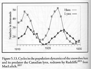
where D_prey and D_predator are the density of prey and predator, respectively, R_prey is the intrinsic rate of prey population increase, a is the predation rate coefficient, b is the replication rate of predators per one prey eaten, and m is the predator mortality rate. When properly parameterized the model can give results that look much like the observed field data of natural populations, such as the cycles in the populations of the Canadian lynx, a predator, and the snowshoe hare, its prey [2857], as shown in Figure 5.13. Interestingly, similar autonomously oscillating populations of microbes have been observed [2858], complete with hysteresis, transients, and a constant final frequency, even for single-species populations in the absence of predator-prey relationships.

There is a vast literature on population ecology [2859-2863] – the branch of ecology that studies the structure and dynamics of populations of replicators – that can provide ideas and guidance for future research on various quantitative aspects of machine self-replication in a variety of circumstances. Topics in population ecology typically include density-dependent and density-independent population growth, age and gender distributions, life history strategies,* spatial dispersal patterns, population invasions and diffusion models, optimal foraging and environmental stress,** territory formation [941] and competitive exclusion, predator-prey interactions (prey is food source), parasite-host interactions (host is food source and habitat), measures of population entropy [443] or community diversity, experimental evolution [2864] and macroevolution [482], and so forth – all of which have their analogs in the design space of mechanical kinematic replicators (Section 5.1.9). However, a complete survey and analysis of the population ecology of machine replicators (e.g., Freitas and Gilbreath [2], Section 5.5.2) is beyond the scope of this book.

* There is a generally-accepted [2625, 2865] spectrum of strategies between two well-recognized extremes: (1) r-selection (high fecundity, rapid development) represents the “quantitative” extreme – in a perfect ecological vacuum with no density effects and no competition, the optimum ecologic strategy is to put all resources into reproduction with the fewest possible resources into each individual offspring, producing as many progeny as possible. (2) K-selection (low fecundity, slow development) represents the “qualitative” extreme – when population density effects are maximal and the environment is saturated with competitors, competition is keen so the optimum ecologic strategy is to put all resources into the maintenance and production of a few extremely fit offspring, leading to increasing efficiency of utilization of environmental resources. As a replicator population grows, reproductive strategy may shift from r-selection (maximum intrinsic rate of natural increase) to K-selection (carrying capacity) [2625].

** For example, during lean conditions the ratio of replicating individuals to the whole population may be reduced in order to preserve the long-living adults for better future times [2866].

Last updated on 1 August 2005